Current Control Simulation by LTspice - The Negligible Lab International

Introduction

When controlling a motor or connecting to the grid by a voltage-source inverter (VSI), current control*1 is necessary. Nowadays, it must be rare to do the job with an analog circuit using operational amplifiers, etc.*2 whereas microcontrollers, DSPs (digital signal processors), and/or FPGAs (field-programmable gate arrays) are chosen as the control hardware. In this case, the system becomes discrete-time where the control computation routine is called cyclically every sampling period like functions called by a timer interruption, etc. A dead time is then introduced for time T so that the control gain design is an issue to ensure stability. Moreover, in the VSI control, PWM converts the output voltage reference to a pulse pattern which has the same average value.

I have learned power conversion circuits and their control. Yet, my understanding to the current control was really ambiguous. Hence, I try to perform the following two comparisons using LTspice XVII and my own control system library, Contraille.

Continous-time (analog) vs. discrete-time (digital) controls
Arbitrary vs. pulse-width-modulated voltage sources

The object here is a simple RL circuit.

f:id:s-inoue2010:20200702023510p:plain:w200 — Fig. 1: RL circuit under study.

The voltage v(t) is adjusted so that the current i(t) has a desired value or waveform. In this case, the "controlled variable" is i(t) whereas v(t) is called the "manipulated variable" although this term seems not widely used. Just in case, t is time and both v(t) and i(t) become a function dependent on time t.

DISCLAIMER: This entry may contain technical errors!

My smattering knowledge heard from others

It is often said (?) that when R = 0 Ω and the sampling period is T, the current i(t) does not overshoot by setting the current control proportional gain K_P to satisfy:

$K_{P} \leq \displaystyle \frac{L}{4 T}. \tag{1}$

This is stated in, e.g., Refs. *3 and *4. However, it could be necessary to pay one's own effort to understand it. So, I will try to play with block diagrams and equations.

Let's see a simulation example.

A schematic shown in Fig. 2 has been created using LTspice XVII and my own control system library, Contraille. There are two controllers, the continuous- and the discrete-time controllers, in parallel, and you can select one by a multiplexer. In addition, one more multiplexer can select whether the output signal of the controller goes directly to the voltage-dependent voltage source E1, or is pulse-width-modulated before going to E1.

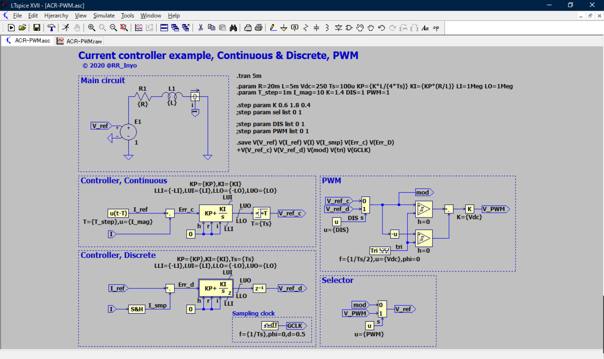
f:id:s-inoue2010:20200702175010p:plain — Fig. 2: LTspice schematic.

This is just an example, but the circuit and control parameters are summerized in Table I.

K \displaystyle \frac{L}{4 T}~[ \mathrm{V/A} ]

K_{P} \displaystyle \frac{R}{L}~[ \mathrm{V/As} ]

Paeameter	Value
Resistor, R	20 mΩ
Inductor, L	5 mH
Sampling period	100 μs
Proportional gain, K_P	$K \displaystyle \frac{L}{4 T}~[ \mathrm{V/A} ]$
Integral gain K_I	$K_{P} \displaystyle \frac{R}{L}~[ \mathrm{V/As} ]$

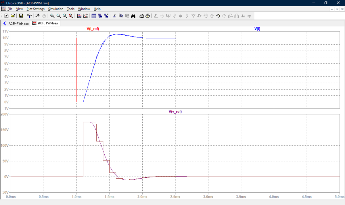
The proportional gain has a parameter K, which is changed to be K = 0.6, 1.0, 1.4, and 1.8, by .step param command of LTspice. When K = 1, K_P = L / (4 T) as in (1).

f:id:s-inoue2010:20200702175120p:plain — Fig. 3: Discrete-time control + PWM

As can be seen in Fig. 3, when K = 1, the current i(t) has no overshoot.

Simple block diagram in continuous time

Fig. 4 shows the simplest block diagram in the s-domain, applying a PI (proportional and integral) controller, the simplest block diagram without considering the dead time.

f:id:s-inoue2010:20200702030157p:plain:w450 — Fig. 4: Continuous-time simple control block diagram

In this case, the open-loop transfer function G_o(s) is:

$G_{o}(s) = \displaystyle \left (K_{P} + \frac{K_{I}}{s} \right ) \frac{1}{s L + R} = \frac{K_{P}}{s L} \frac{s + \frac{K_{I}}{K_{P}}}{s + \frac{R}{L}} \tag{2}.$

If you set the proportional gain K_P and the integral gain K_I to satisfy:

$\displaystyle \frac{K_{I}}{K_{P}} = \frac{R}{L} \tag{3},$

pole-zero cancellation occurs, making G_o(s) be:

$G_{o}(s) =\displaystyle \frac{K_{P}}{s L} \tag{4}.$

Then, the closed-loop transfer function G_c(s) is a first-order delay with ω_n = K_P / L as expressed like:

$G_{c}(s) = \displaystyle \frac{\frac{K_{P}}{L}}{s + \frac{K_{P}}{L}} \tag{4}.$

The problem here is how the proportional gain K_P should be set. As mentioned above, if setting K_P = L / (4 T), which is the border to have no overshoot,

$G_{c}(s) = \displaystyle \frac{\frac{1}{4 T}}{s + \frac{1}{4 T}} \tag{5}.$

This is a first-order delay of ω_n = 1 / (4 T). For example, if T = 100 μs, ω_n = 2,500 rad/s.

In reality, however, a dead time accompanying the computational time and frequency characteristics of the current sensor matter so that it is necessary to check the gain and phase margins, (which I would like to write in another entry.)

Block diagram in discrete-time control

As far as I see some textbooks, they first express discrete-time control systems in the continuous-time s-domain. Let's begin with R = 0 Ω and K_I = 0.

f:id:s-inoue2010:20200702142954p:plain:w600 — Fig. 5: Block diagram expressing discrete-time control in the s-domain.

In Fig. 5, e^−sT is a dead time for one sampling period and (1 − e^−sT) / s is the transfer function of a zero-order hold. The open-loop transfer function G_o(s) is derived from Fig. 5 as:

$G_{o}(s) = \displaystyle \frac{(K_{P} / L) (e^{-s T} - e^{-2 s T})}{s^{2}} \tag{8}.$

Converting this to the z-domain, you obtain:

$G_{o}(z) = \mathcal{Z} [G_{o}(s) ] = \displaystyle \frac{(K_{P} T / L) z (z^{-1} - z^{-2})}{(z - 1)^{2}} = \frac{K_{P} T / L}{z (z - 1)} = \frac{K_{P} T / L}{z^{2} - z} \tag{8}.$

The closed-loop transfer function G_c(z) can be written as:

$G_{c}(z) = \displaystyle \frac{G_{o}(z)}{1 + G_{o}(z)} = \frac{K_{P} T / L}{z^{2} - z + K_{P} T / L} \tag{9}.$

Then, the characteristic roots of G_c are:

$z = \displaystyle \frac{1}{2} \pm \sqrt{\frac{1}{4} - \frac{K_{P} T}{L}} \tag{10}.$

The overshoot does not happen when the characteristic roots are real. It means that the inside of square root in (10) is positive as follows:

$K_{P} < \displaystyle \frac{L}{4 T} \tag{11}.$

This is the way to theoretically reach the conclusion of "My smattering knowledge heard from others" (although I do not fully understand how...😅).

Simulation results

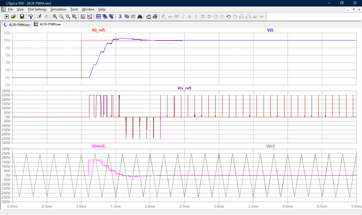
Let me present other simulation results.

f:id:s-inoue2010:20200702182326p:plain — Fig. 6: Continuous-time + no PWM

f:id:s-inoue2010:20200702182423p:plain — Fig. 7: Continuous-time + PWM

f:id:s-inoue2010:20200702182523p:plain — Fig. 8: Discrete-time + no PWM

I will prepare and clean up my own control system library Contraille and make it available publicly!

[Updates while translating] I have uploaded Contraille in GitHub already. See below.

github.com

Updates: Moving-average filter to detected current signal

The continuous-time controller in Fig. 2 compared the detected current signal directly with the current reference. Meanwhile, the discrete-time controller needed to sample and hold the current signal i(t) after detection. I guessed that the difference between continuous- and discrete-time controller in Figs. 3 and 6-8 was in this point.

Textbooks of digital control and z-transform say transfer function of sample and hold, G_SH(s), can approximately be written as:

$G_{\mathrm{SH}}(s) = \displaystyle \frac{1 - e^{-s T}}{s T} \tag{12}.$

This is completely the same as that of the moving average filter (MAF). Hence, why don't we add a MAF to the detected current signal i(t) in the continuous-time controller and compare its behavior with that of the discrete-time controller again?

f:id:s-inoue2010:20200703013146p:plain — Fig. 9: Adding a moving-average filter to the detected current signal in the continuous-time controller.

Let's set the current control proportional gain K_P = 1.4 × L / (4 T) which will cause overshoot and compare the continuous- and discrete-time controllers.

f:id:s-inoue2010:20200703013448p:plain — Fig. 10: Continuous-time controller with a MAF and discrete-time controller (without PWM)

f:id:s-inoue2010:20200703013542p:plain — Fig. 11: Continuous-time controller with a MAF and discrete-time controller (with PWM)

Whoa! Waveforms of continuous- and discrete-time controllers almost perfectly coinside! Adding a MAF to the continuous-time controller has made the behaviors of the two controllers almost equal, whereas they were different in Figs. 3 and 6-8 despite the same proportional gain K_P. In other words, discrete-time (digital) control, needing to perform sample and hold, automatically has a characteristics of MAF in the feedback loop. In addition, this coincidence does not depend on whether PWM is done or not.

Well, I had not been able to deeply grasp this kind of insight without doing hands-on myself.

Appendix

This is a translation to my original Japanese entry linked below:

negligible.hatenablog.com

*1:Sometimes current control is referred to as "ACR", but I guess this is a Japanese English.

*2:早川：「初めての自立移動ロボット制御シミュレーション」，トランジスタ技術，2020年7月号，pp. 71-86

*3:J. Tahara, H. Fujita, and H. Akagi, "Control and performance of a PWM eectifier with an FPGA-based current controller," IEEJ Technical Meeting on Semiconductor Power Converter, SPC-05-14, Jan. 2005, Osaka, pp. 33-38.
田原・藤田・赤木：「FPGAによる高速電流制御を適用したPWM整流器の動作特性」，電気学会半導体電力変換研究会資料SPC-05-14，pp. 33-38，2005年1月，大阪

*4:H. Akagi, E. H. Watanabe, and M. Aredes, Instantaneous Power Theory and Applications to Power Conditioning, Wiley, 2007